
An Introduction to Compilers
This blog post introduces the world of compilers with an example in Golang. The code comes from the book Writing An Compiler In Go by Thorsten Ball.
Post Outline
Introduction
In this blog post we will be covering the main parts of writing a compiler. The post is divided into two main parts: background (where I go over the basic outline and details of compilers) and code (where I bring up specific examples from the book Writing a Compiler in Go).
Background
How do compilers work
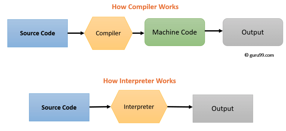
In general, compilers take in source code and output machine code that can be executed on a specific architecture. More specifically, compilers take in source code and parse it into an AST (abstract syntax tree as covered in a previous blog post) using a lexer and a parser. The AST is then converted into an intermediate representation upon which several optimization passes are applied to. Then a code generator outputs the target machine code. There are many more steps involved but these ones cover the major parts.
How do compilers compare to interpreters
Interpreters, like compilers, are another common kind of language processor. Both will have the same front end where the source code is lexed and parsed into an abstract syntax tree (AST). After the AST is where the paths diverge. An interpreter directly executes the operations specified in the source program on user supplied inputs A compiler, on the other hand, produces a target program in the target language that is executed when the user supplied inputs.
A compiler-produced program is typically much faster than an interpreter because the machine code from the compiler program is optimized for the specific architecture. On the other hand, an interpreter can be much better at providing error messages that are language specific to the source code because there isn’t the source/target language abstraction layer that the compiler has.
What about languages that are both compiled and interpreted
There are many popular languages like Java and Python that are both compiled and interpreted.
The source program in these languages is first compiled into an intermediate program represented in bytecode. The bytecode is then interpreted using a processor virtual machine.
Because of the two separate components to the overall process, the bytecodes can be compiled on one machine and interpreted on another, introducing some flexibility.
Virtual machines
Let’s go into more detail about the processor virtual machine.
Note that the processor virtual machine (like JVM) is different from a system virtual machine (like a VMware product). A system virtual machine is a program that emulates a computer, including the disk drive, hard drive, graphics card, and more. A processor virtual machine is used to implement programming languages and are used to emulate the behavior of the hardware. They can be thought of as the software equivalent of the hardware. More detail can be found in this wikipedia article.
Hardware: the von Neumann architecture
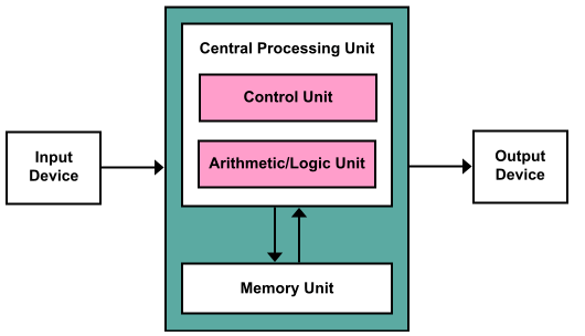
What exactly is the hardware that a processor virtual machine is mimicking? The hardware that is being mimicked, while varying depending on the brand and model, typically follows the von Neumann architecture.
The von Neumann architecture has the following parts:
- CPU
- processing unit: ALU + Processor Registers
- control unit: instruction register, program counter
- Memory (RAM)
- Mass storage (hard drive)
- input/output devices
The CPU (i.e. the central processing unit) is made up of two parts: the processing unit and the control unit. The processing unit has the ALU (arithmetic logic unit) and multiple processor registers. The control unit has a instruction register (holds current instruction being executed) and a program counter (keeps track of next instruction to execute). The CPU performs “basic arithmetic, logic, controlling, and input/output operations specified by the instructions in the program” (Source). The memory (Random Access Memory) stores the program’s data and instructions. There is also mass storage in the form of hard drives and disks that make up non volatile memory. Then there are input/output devices like the keyboard and the display.
CPU
The CPU performs a constant fetch, decode, execute cycle.
When a CPU is measured in megahertz, it refers to the frequency of this cycle (i.e. how many cycles in a particular time frame). During the fetch phase, an instruction is fetched from memory using the program counter. During the decode phase, an instruction is decoded, meaning that the computer determines which operation should be executed based off of the instruction. In the execute phase, the instruction is executed. This can mean that the values stored inside of registers is modified, that data is transferred from a register to memory, that data is moved around in memory, that output is generated, that input is read, and more.
Memory
So the CPU uses a program counter to keep track of where to fetch the next instruction. The program counter’s value is an address that points to somewhere in memory.
Memory is organized into groups of bytes called words. The size of the word varies depending on the architecture. Typically 32 and 64 bit word sizes are used in modern computers.
There is also a memory region called the call stack, or just the stack. This region is where the CPU performs LIFO (last in first out) operations on. The call stack holds the return address, local variables, and function arguments. A stack data structure is chosen because it plays well with nested function calls. The pushing and popping of instructions fit how functions call one another before returning to their caller. This blog post goes into more detail about the calling conventions, specifically on the x86 architecture.
CPUs also have processor registers to store data. This is a step up from the memory hierarchy from RAM. It is much faster but has significantly less storage space, much like how RAM compares to disk. In an x86-64 architecture, the CPU has 16 general purpose registers holding 64 bits of data each. Registers are used for data that is used very frequently, such as a pointer to the next instruction to execute in the stack (i.e. the stack pointer).
Physical Machine to Virtual Machine
Now that we know what the virtual machine is emulating, lets see how the virtual machine mimics the hardware. The virtual machine has a fetch decode execute cycle just like the CPU. It also has a program counter that points to the next instruction to execute. There is also a call stack and multiple registers.
An example of a processor virtual machine is the Java Virtual Machine (JVM).
Stack based VM vs Register based VM
There are two broad categories of virtual machines: stack based virtual machines and register based virtual machines.
A stack based virtual machine is a virtual machine that relies completely on its call stack to perform all operations. A register based virtual machine is a virtual machine that has a call stack and registers. Instructions can use the registers in addition to the stack. This results in less instructions compared to the stack based VM because we don’t need to push/pop everytime to perform a computation. However, a register based machine is more complicated to implement simply because it has more pieces (i.e. the registers) in addition to the call stack.
The compiler in the book
The code is from the book’s Monkey language and is written in Golang.
The compiler uses a stack based virtual machine.
Concrete Code
The following sections show concrete code from the compiler.
Bytecode
The code shown is for a compiler using a stack based virtual machine. As mentioned previously, source code is compiled into bytecode and interpreted by the virtual machine to be executed. Bytecode can then be thought of as instructions that tell the virtual machine what to do.
The instructions, represented by opcodes, in the bytecode are each one byte in size. In addition, the operands (parameters to the opcodes) are also represented by bytes.
We can see this in the Opcode and Instructions definitions in Monkey.
type Instructions []byte
type Opcode byte
Now that we’ve defined the type of an Opcode, lets see how actual opcodes are defined. The OpCode definitions are a map with an OpCode byte being the key and the definition being the value. A Definition type is defined to eb made up of the name of the operand (e.g. PUSH) and the number of bytes each operand takes up in OperandWidths.
type Definition struct {
	Name          string
	OperandWidths []int
}
For instance, the OpConstant operator, representing an integer, can be added to the definitions map like so:
var definitions = map[Opcode]*Definition{
    ...
	OpConstant: {"OpConstant", []int{2}},
    ...
}
The operand is 2 bytes wide, indicating that it is of type uint16.
Based off a given OpCode, there will be a function that creates the corresponding bytecode.
The function Make() takes in an opcode and its corresponding operands and returns a byte array representing the bytecode.
The function works by looking up the opcode in the definition.
It then creates a byte array where the first value is the opcode and the rest are any operands.
func Make(op Opcode, operands ...int) []byte {
	def, ok := definitions[op]
	if !ok {
		return []byte{}
	}

	instructionLen := 1
	for _, w := range def.OperandWidths {
		instructionLen += w
	}

	instruction := make([]byte, instructionLen)
	instruction[0] = byte(op)

	offset := 1
	for i, o := range operands {
		width := def.OperandWidths[i]
		switch width {
		case 2:
			binary.BigEndian.PutUint16(instruction[offset:], uint16(o))
		case 1:
			instruction[offset] = byte(o)
		}
		offset += width
	}

	return instruction
}
Endianess
Note that we can order the bytecode in one of two ways: left to right or right to left in terms of least significant to most significant bit. Different architectures order the bytecode in one of the two ways.
Compiler and Virtual Machine
So we now know how bytecode is represented and created from opcodes and their operands (i.e. assembly). The compiler generates the bytecode from the parsed program. Let’s first take a look at repl, which takes in a program, parses it into an AST as covered in the interpreter blog post, and compiles it. The bytecode is then passed to the virtual machine, which interprets the bytecode. This is shown in the following code:
func Start(in io.Reader, out io.Writer) {
	scanner := bufio.NewScanner(in)

	for {
		fmt.Printf(PROMPT)
		scanned := scanner.Scan()
		...

		line := scanner.Text()
		l := lexer.New(line)
		p := parser.New(l)

		program := p.ParseProgram()
		...

		comp := compiler.New()
		err := comp.Compile(program)
		...

		machine := vm.New(comp.Bytecode())
		err = machine.Run()
		...

		stackTop := machine.StackTop()
		io.WriteString(out, stackTop.Inspect())
		io.WriteString(out, "\n")
	}
}
Compiler
The compiler has a Compile(program) function that parses the AST nodes and emits the respective bytecode.
There is a switch statement for all the possible AST nodes.
An example with a constant is shown below:
func (c *Compiler) Compile(node ast.Node) error {
	switch node := node.(type) {

    ...

	case *ast.IntegerLiteral:
		integer := &object.Integer{Value: node.Value}
		c.emit(code.OpConstant, c.addConstant(integer))

    ...

	return nil
}
The compiler’s emit function calls the bytecode Make() function (shown previously) and appends the resulting bytes to the compiler’s array of bytes instructions representing all the bytecode compiled so far.
Virtual machine
The key part of the virtual machine is the fetch decode execute cycle performed that mimics the hardware CPU.
This is encapsulated in the Run() function.
The VM loops through all the instructions using the instruction pointer ip and fetches the current instruction.
The instruction is then decoded using the switch/case statement.
In the below code, the OpConstant case is shown.
The instruction is executed by parsing the constant out of the bytecode and pushing it onto the virtual machine’s stack.
func (vm *VM) Run() error {
	for ip := 0; ip < len(vm.instructions); ip++ {
		op := code.Opcode(vm.instructions[ip])

		switch op {
		case code.OpConstant:
			constIndex := code.ReadUint16(vm.instructions[ip+1:])
			ip += 2

			err := vm.push(vm.constants[constIndex])
			if err != nil {
				return err
			}

        ...
	}

	return nil
}
Compiling Expressions
Now let’s see how Monkey compiles and interprets the infix add expression (e.g. 5 + 3).
There are two parts to adding this functionality: in the compiler and in the virtual machine.
Compiler
In the compiler, we need to generate the bytecode corresponding to this infix expression.
We can simply add the follwoing case to the compiler’s Compile() function while its parsing the AST:
case *ast.InfixExpression:
    ...
    err = c.Compile(node.left)
    ...
    err = c.Compile(node.Right)
    ...
    case "+":
        c.emit(code.OpAdd)
    ...
First the Compile function recursively calls itself on either side.
This is because our VM’s add operation will operate on the previous two expressions appended to the stack.
The above code then calls emit(), which uses the Make() function and Definitions map we mentioned previously to generate the proper bytecode (using the OpAdd’s unique opcode).
Virtual Machine
In the virtual machine is where we parse the OpAdd. We can do this in the fetch decode execute cycle in run by simply adding another case:
case code.OpAdd:
    right := vm.pop()
    left := vm.pop()
    leftValue := left.(*object.Integer).Value
    rightValue := right.(*object.Integer).Value

    result := leftValue + rightValue
    vm.push(&object.Integer{Value: result})
This code pops the top two elements from the stack, adds them together, then pushes them back on.
Conditionals
Let’s see how the compiler and virtual machine compile the source code and interpret the resulting bytecode for conditional statements (i.e. if statements).
Compiler
When the source program has an if statement, the front end of the compiler (i.e. the lexer and parser) construct the abstract syntax tree with an IfExpression node representing the conditional.
In our compiler’s Compile() function, we can add a new case for our switch statement as we’re traversing the AST.
case *ast.IfExpression:
    err := c.Compile(node.Condition)
    if err != nil {
        return err
    }

    // Emit an `OpJumpNotTruthy` with a bogus value
    jumpNotTruthyPos := c.emit(code.OpJumpNotTruthy, 9999)

    err = c.Compile(node.Consequence)
    if err != nil {
        return err
    }

    if c.lastInstructionIs(code.OpPop) {
        c.removeLastPop()
    }

    // Emit an `OpJump` with a bogus value
    jumpPos := c.emit(code.OpJump, 9999)

    afterConsequencePos := len(c.currentInstructions())
    c.changeOperand(jumpNotTruthyPos, afterConsequencePos)

    if node.Alternative == nil {
        c.emit(code.OpNull)
    } else {
        err := c.Compile(node.Alternative)
        if err != nil {
            return err
        }

        if c.lastInstructionIs(code.OpPop) {
            c.removeLastPop()
        }
    }

    afterAlternativePos := len(c.currentInstructions())
    c.changeOperand(jumpPos, afterAlternativePos)
So what’s going on in the above code?
First, the condition is compiled by calling Compile() recursively.
This condition should evaluate into true or false value that is then emitted from the compiler.
Then an OpJumpNotTruthy opcode is emitted. This is a simple OpCode that tells the virtual machine to jump to a different offset in the instructions if the previous value in the stack is not true. This prevents the block of statements inside the if to be executed if the condition is false.
Then the consequence of the node is compiled by calling Compile() recursively.
The consequence is what is executed if the if statement conditional was true.
If the if statement conditional was true then the OpJumpNotTruthy would not cause the virtual machine’s instruction pointer to jump and would instead execute the consequence bytecode.
Then the OpJump bytecode is emitted.
At this point, we want to jump over the bytecode to be loaded in next (i.e. the code in the else statement if one exists, called the node’s alternative).
After this we change the operand to the OpJumpNotTruthy because we want to jump to after the OpJump bytecode right before the alternative field to be compiled next. We could only calculate the offset after the OpJump bytecode was created so as to know how far to jump to after that op.
We then emit the bytecode for the node’s alternative field, which can be NULL if there is no else statement.
We then change the operand (parameter) to the OpJump to be the current location (now that we know the offset of the bytecode up until this point). We had to change the operand after the alternative was compiled so we could know how much to jump so as to land right after the alternative.
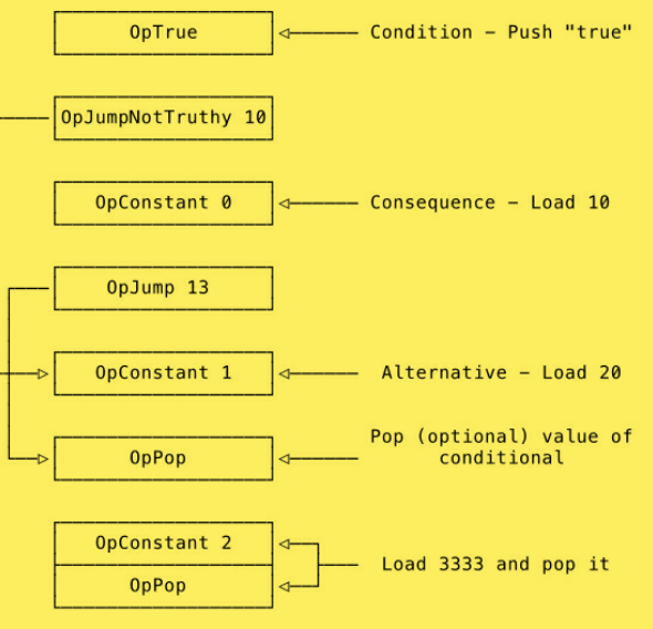
The below picture taken from the book illustrates the bytecode that is generated from a simple if/else conditional statement.
Virtual Machine
The main parts of the virtual machine that have to do with conditionals are interpreting the OpJump and OpJumpNotTruthy opcodes. Essentially two cases are added to the switch statement that performs the decoding of the VM’s fetch decode execute cycle.
case code.OpJump:
    pos := int(code.ReadUint16(ins[ip+1:]))
    vm.currentFrame().ip = pos - 1

case code.OpJumpNotTruthy:
    pos := int(code.ReadUint16(ins[ip+1:]))
    vm.currentFrame().ip += 2

    condition := vm.pop()
    if !isTruthy(condition) {
        vm.currentFrame().ip = pos - 1
    }
In the case of the OpJump code, we simply read in the operand and set the instruction pointer to be that operand.
In the case of hte OpJumpNotTruthy opcode, we initially assume that the condition is true and set the instruction pointer to be after the current opcode and operand.
Then we check the condition and if its not truthy, then we set the instruction pointer to be at that position.
The -1 of the position is an implementation detail resulting from the fetch decode execute cycle in Run() incrementing the instruction pointer by 1 every iteration.
Symbol Table
Now let’s talk about how to implement variables in our compiler. The main idea is to add a symbol table to the compiler that stores all the variables defined by the user program. Then the virtual machine can interpret the special bytecode for the variables that the compiler generated.
Compiler
There are two situations with variables. The first is when a variable is defined. In the AST, this is represented with a let statement. Let’s start by adding a new case for the let statement in our Compile function’s switch statement.
case *ast.LetStatement:
    symbol := c.symbolTable.Define(node.Name.Value)
    err := c.Compile(node.Value)
    ...

    ...
        c.emit(code.OpSetGlobal, symbol.Index)
    ...
Let’s analyze the above code.
First, a new entry is added to the symbol table using the Define() function.
This function assigns a new unique index to each variable that comes in.
The bytecode for the value of the variable is then generated by recursively calling Compile() on the value.
Then the bytecode for the OpSetGlobal is defined.
The way the opcode OpSetGlobal works is that it has a single operand that is the unique index of the value.
As we’ll see later on, when the virtual machine sees the OpSetGlobal op, it will assign to the unique index the value at the top of the stack.
For now we can see that the compiler emits the bytecode for the value and then the bytecode for the OpSetGlobal op.
Next is the case where we see a symbol in the user program and we need to resolve it (i.e. figure out the value).
We can add a new case to the Compile() function - the identifier case.
This is the way the AST represents a variable that it encounters when parsing the user program.
The way this function works is that it resolves the node’s value via the symbol table.
The Resolve() function simply looks up the variable in the symbol table and returns it if it exists.
case *ast.Identifier:
    symbol, ok := c.symbolTable.Resolve(node.Value)
    ...

    c.loadSymbol(symbol)
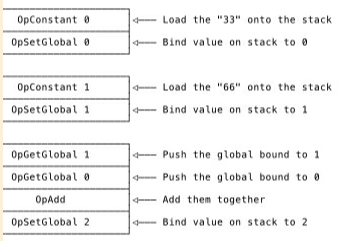
The following is the bytecode generated.
Virtual Machine
Now that the bytecode from the compiler has been emitted, let’s see how the virtual machine interprets them. When the virtual machine encounters the OpSetGlobal op in the bytecode, it first reads in the operand of the op to get the unique index corresponding to the value. It then creates a new entry in the globals map representing the global variables with the index as the key and the next value in the stack as the value to be set.
case code.OpSetGlobal:
    globalIndex := code.ReadUint16(ins[ip+1:])
    vm.currentFrame().ip += 2

    vm.globals[globalIndex] = vm.pop()
When the virtual machine encounters an OpGet, this means that it has encountered a usage of a particular variable. We can simply decode the operand of the operator representing the unique index corresponding to the variable. We then increment the instruction pointer by 2 to get past the operand and then push the value assigned to the variable onto the stack.
case code.OpGetGlobal:
    globalIndex := code.ReadUint16(ins[ip+1:])
    vm.currentFrame().ip += 2

    err := vm.push(vm.globals[globalIndex])
    ...
Compiling Functions
To implement function calls, we want to emit bytecode instructions that represent Monkey’s calling convention. Calling convention is a scheme for how functions call one another. In a previous blog post we saw how calling conventions for x86 worked. Once the bytecode is emitted, we want the virtual machine to actually execute the instructions.
Compiler
On the compiler side of things, we can add three new cases to the switch statement in Compile() while traversing the AST.
The first is the ast.CallExpression:
case *ast.CallExpression:
    err := c.Compile(node.Function)
    if err != nil {
        return err
    }

    for _, a := range node.Arguments {
        err := c.Compile(a)
        if err != nil {
            return err
        }
    }

    c.emit(code.OpCall, len(node.Arguments))
This is what is first encountered in the ast during a function call.
The case recursively calls Compile() on the node’s functions and all the nodes arguments.
Then bytecode is emitted for the op OpCall.
When the actual function is called, we hit the ast.FunctionLiteral case.
case *ast.FunctionLiteral:
    ...

    for _, p := range node.Parameters {
        c.symbolTable.Define(p.Value)
    }

    err := c.Compile(node.Body)

    ...

    compiledFn := &object.CompiledFunction{
        Instructions:  instructions,
        NumLocals:     numLocals,
        NumParameters: len(node.Parameters),
    }
    c.emit(code.OpConstant, c.addConstant(compiledFn))
In the above, we define the parameters in the symbol table and compile the node body. Then a constant is returned representing the unique index of the function.
When the body of the function is being compiled, it will hit a return statement. In the following case, the return value is compiled and placed onto the stack if not null. Then the OpReturnValue code is emitted.
case *ast.ReturnStatement:
    err := c.Compile(node.ReturnValue)
    ...

    c.emit(code.OpReturnValue)
Virtual Machine
The virtual machine has the job of interpreting and executing the bytecode given by the compiler.
Let’s see how the virtual machine executes the function bytecode it is given.
We add two cases to the virtual machine’s fetch decode execute loop in Run().
The first is for OpCall.
The arguments are read in and passed into the helper callFunction.
case code.OpCall:
    numArgs := code.ReadUint8(ins[ip+1:])
    vm.currentFrame().ip += 1

    err := vm.callFunction(int(numArgs))
    ...
The helper function access the CompiledFunction from the value stored on the stack representing the unique index of the function. A new frame representing the scope of the function is pushed onto the stack.
func (vm *VM) callFunction(numArgs int) error {
	fn, ok := vm.stack[vm.sp-1-numArgs].(*object.CompiledFunction)
	...

	frame := NewFrame(fn, vm.sp-numArgs)
	vm.pushFrame(frame)

	vm.sp = frame.basePointer + fn.NumLocals

	return nil
}
The stack pointer is updated and the function returns as the fetch decode execute cycle continues and executes the function body. This continues until the return statement from the function is hit. At this point, the return value is popped off of the stack as well as the stack frame that was pushed during the function call. The return value is then pushed back onto the stack for future use by the user program.
case code.OpReturnValue:
    returnValue := vm.pop()

    frame := vm.popFrame()
    vm.sp = frame.basePointer - 1

    err := vm.push(returnValue)
    ...
Conclusion
In this blog post we covered basic concepts in compilers, specifically compilers that use virtual machines to interpret compiled bytecode.
These concepts were illustrated through the Monkey language from the book Writing a Compiler in Go with code examples on how bytecode is generated, how expressions, conditionals, and functions are compiled, and how variables are implemented.