
Semi Supervised Learning for Time Series Classification
An investigation in applying pseudo labeling, a common technique in semi supervised learning where we have limited labeled data, to time series classification.
Post Outline
- Pseudo Labeling and Semi Supervised Learning
- Time Series Classification
- Pseudo Labeling Experiments
- Iterative Pseudo Labeling
- Resources
Pseudo Labeling and Semi Supervised Learning
Pseudo labeling in deep learning is like a student taking a class on a topic and after the class is over, learning more about it on his/her own.
As a concrete example, let’s say we wanted to learn to distinguish between a cat and a dog, neither of which we have seen before. However, we do have a single picture of each. We then have a pile of pictures that we know are either cats or dogs but don’t know which.
We can imagine our data as in the following diagram. The clear circle represents “cats”. The shaded circle represents “dogs”. The gray circles represent our unlabeled data. The dotted line represents the boundary that separates the two classes.
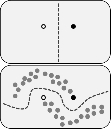
Now, given an unlabeled picture, the natural thing to do would be to compare our two labeled pictures with that unlabeled picture. We might guess that it is a dog because it has a similar nose to the labeled dog picture.
The above is an example of pseudo labeling. Pseudo labeling is like someone with some prior knowledge about a topic learning knew material and using that newly learned material with all the prior knowledge to learn even more. This technique lies in the realm of semi supervised learning, where we have a small amount of labeled data and a ton of unlabeled data. This field is very useful in deep learning because deep learning models require lots and lots of data to achieve reasonable accuracies for tasks and depending on the task (which might be very specific), the amount of labeled data required to achieve a reasonable accuracy may not be feasible to acquire.
More formally, pseudo labeling is where we train a classifier on a small amount of labeled data to generate “pseudo labeled” data. We then train a new classifier on the original labeled data and pseudo labeled data, ideally creating an even better classifier that can perform better than a classifier trained solely on the tiny labeled dataset.
Time Series Classification
Now that we’ve covered pseudo labeling, let’s take a look at a particular domain that we can apply pseudolabeling to: time series classification (TSC).
Let’s say we have data measuring heartbeats over a specific time period and we know that certain patterns of heartbeats are indicative of particular problems (e.g. arrhythmia). For example, a patient with a heart murmur may have a significantly different looking time series chart than a patient without the condition. In TSC, we are given examples of time series that can be classified under different labels and are asked to determine the class of an unlabeled time series.
Formally, TSC data can be described as below:
\[X = (x_1, x_2, ..., x_T)\]The subscript $T$ is the length of the time series (i.e. how long the measurement was taken for). The above is an example of a univariate time series where there is a single data point for each time step. We may also have multivariate time series where there are multiple data points for each time step. A $d$ dimensional multivariate dataset looks like:
\[X_i = (x_1, x_2, ..., x_d)\]We have an $X_i$ for each $i \in 1, …, T$. We then have a label $Y$ for each class. Our goal is to learn a function of the form:
\[f: X \rightarrow Y\]Pseudo Labeling Experiments
Methodology
The following is the pseudocode for pseudolabeling on a particular dataset. A ResNet model is used.
- Split up the training data into 2 parts
- Train ResNet on the first part
- Generate pseudolabels on the second part
- Combine pseudolabels of second part and labels of first part as labels
- Train new ResNet model on the combined dataset
Results
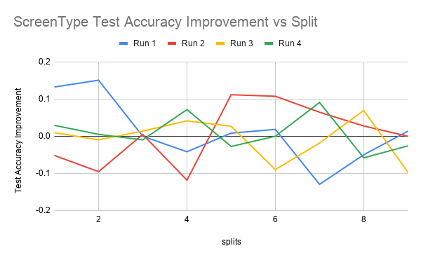
Here are the results from training on the ScreenType dataset.
Note that the training data is split into labeled and unlabeled portions. The experiments ran where the fraction of labeled training data ranged from 1/10, 2/10, … 9/10. A “split” is defined as a number associated with the fraction of the training data that is labeled. So for example if we had 3/10 labeled training data our “split” would be 3.
The first figure shows test accuracy improvements for 4 runs over every split from 1 to 10. The second figure shows the mean and median test accuracy improvement. Test accuracy improvement is defined as the percentage improvement of the classifier trained on both labeled and pseudolabeled data (aka the student model) over the classifier trained just on the labeled data (aka the teacher model) on the test data set.
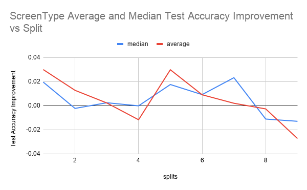
From ScreenType Average and Median graph, we can see that the student model improves upon the teacher model with the pseudolabels in split 1 and between splits 4 and 8. It seems like the initial increase is due to the fact that given that the size of the training data is only 375 examples, the teacher’s accuracy is only based off of 37 examples. Because this amount of labeled data is so small, it could be that the additional pseudolabeled data seen by the student, even if it’s quality is not as good as labeled data, is beneficial enough to increase the test accuracy.
It can be seen that there is improvement for the splits between 4 and 8 in the Average and Median graph for both ScreenType. It could be that that this is because there is some optimal split fraction in this range where we have enough labeled data to generate pseudolabels of reasonable quality but also not so much high quality labeled data where any more pseudolabeled data that we add would not be helpful anymore as we are already hitting the ceiling of what test accuracy a model trained on the full labeled dataset would achieve.
Iterative Pseudo Labeling
Iterative pseudolabeling means performing pseudo labeling over multiple iterations.
Let’s go back to our cat/dog example for pseudolabeling. We have classifier the unlabeled picture as a dog. We now have a better understanding of what a dog looks like in a different context (e.g. different lighting, posture, etc.). Let’s say that the next unlabeled picture is also a dog and the shape of its head is similar to the first unlabeled image. Given the first unlabeled image, which we determined was a dog from our labeled image, we can determine that the second unlabeled image is also a dog (when we might not have with just the labeled image).
Methodology
Here is some pseudocode.
- Train a teacher model on the labeled data to generate pseudolabels for unlabeled data
- Train a student model using both labeled data and pseudolabeled data
- Make student the teacher to generate new pseudolabels and train a new student model and iterate steps 1 and 2 a certain number of times
Results
Here are the results on another dataset, ElectricDevices.
The data is run over 4 splits: 2, 4, 6, and 8. Each split is run for three iterations.
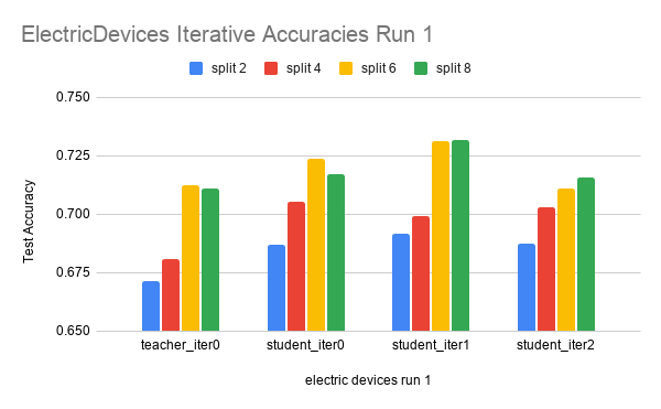
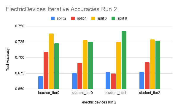
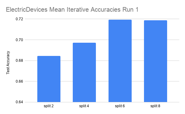
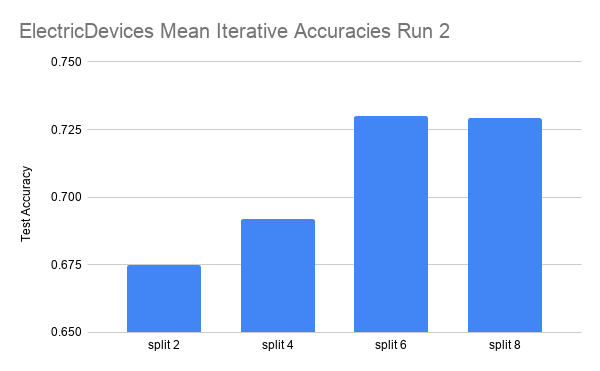
In the ElectricDevices figures, it is important to keep in mind that this dataset is many orders of magnitude larger than ScreenType. Having more data means being able to generalize better by making higher quality pseudolabels, especially when the amount of labeled training data used is limited to a very small subset of the original training data. We can see that we reach the point of diminishing returns in both runs between split 6 and split 8. At this point, we believe that this signals that the splits have hit the point where any more pseudolabels being added would only hinder the test accuracy performance because we are already using most of the original labeled data. Any more labeled data that is not high quality (i.e. the original labeled data) will have either no effect or even an adverse effect as seen in this case.