SIR Model From Scratch in Python
This post explains the SIR model and includes a Python implementation that generates a graphic describing a population’s infectious status over time.
Post Outline
Explanation
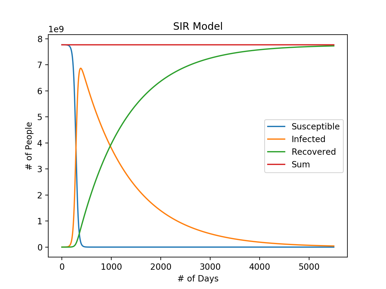
SIR modeling is a method of tracking the progression of an infectious disease over time. The population in the model is separated into 3 disjoint groups: susceptible, infected, and recovered. Initially, there is an infected population that infect more and more of the susceptible population. Infected people also recover, moving from the infected population to the recovered population.
The changes in population for each of the 3 groups can be modeled through differential equations. Here is the source of the below image.
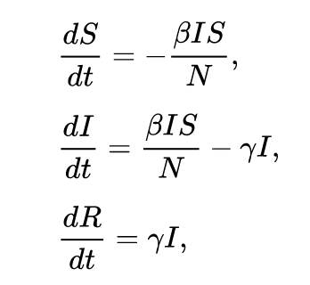
The variables I, S, and R represent the population count of each group while N represents the total population count. The parameter beta controls how often a susceptible-infected contact results in a new infection. The parameter gamma represents the rate an infected recovers and moves into the resistant phase. At each time step dt, each population group is changed by an amount determined by each of those equations.
Code
The full script can be found in this repo. We make several assumptions in our implementation:
- no new additions to susceptible group
- population changes only as a result of the current disease
- fixed # of people will recover any given day
- once recovered, can’t get reinfected
We also predefine several variables:
- init_infected: initial # of people infected
- beta: The parameter controlling how often a susceptible-infected contact results in a new infection
- gamma: The rate an infected recovers and moves into the resistant phase
- iterations: how many steps to run the simulation for
- population_size: total # of people in the model’s world
Our code models the populations over a predefined number of iterations. At each iteration, we append the size of each group at the next iteration to its respective list. The three resulting lists representing the count of the susceptible, infected, and recovered populations are shown together in the final graph.
// Predefined number of iterations
for i in range(iterations):
        // Calculate change in size of each subgroup of the population
        dS = - beta * (susceptible[i] / population_size) * infected[i] * delta_time
        dR = gamma * infected[i] * delta_time
        dI = -dS - dR

        // Append to output list
        susceptible.append(susceptible[i] + dS)
        recovered.append(recovered[i] + dR)
        infected.append(infected[i] + dI)
Note that each of the outputs of the differential equations calculated are multiplied by a variable delta_time. This variable represents the change in time at each time step dt. Looking at the differential equations described in the Explanation section, we see that we can get dS, dI, and dR by multiplying both sides by dt. The smaller the value of dt, the greater the accuracy. In calculus, this is taking the derivative of a variable. We are approximating the derivative by calculating the change in R over a change in t (also known as the slope).
Running the following command will generate the graph.
python3 SIR_model.py