An exploration of pseudo random number generators and their applications in sampling.

Post Outline

• What Are Pseudo Random Number Generators
• Multiplicative Congruential Generators
• How to Sample
• Conclusion

What Are Pseudo Random Number Generators

Often in computing we want to generate random numbers. For example, quick sort is an algorithm that relies on well-randomized subsequences to achieve $O(n \log n)$ expected run time. Another example lies in sampling from distributions, which will be covered in this post.

Pseudo random number generators can be thought of as a machine that, given some inputs, will produce a sequence of numbers that look random but are in fact deterministic, hence “pseudo random”. The most important input to any pseudo random number generator is a number called a “seed”. Different seeds provide different sequences of numbers. The same seed will provide the same sequence of numbers.

Multiplicative Congruential Generators

This post will cover a particular pseudo random number generator: Multiplicative Congruential Generators. Multiplicative Congurential Generators take as input three numbers: a large prime $m$, a multiplier $a \in 2, 3, …,m-1$, and a seed $R_0 \in 1, 2, …, m-1$. Multiplicative Congurential Generators generate the next number in a pseudo random sequence based on the previous value starting with the seed via the following recurrence relation.

The sequence $R_0, R_1, …$ is then a sequence of pseudo random numbers with values between $1$ and $m-1$ inclusive. MCGs generate every number between $1$ and $m-1$ in the first $m-1$ samples. Each following set of $m-1$ cycles start over from $R_0$, which can be proved by Fermat’s Little Theorem (shown below). For example, if $m = 4$ and the sequence of samples we generated was $3, 1, 2$, we could continuously get $3, 1, 2, 3, 1, 2, …$ over and over again. This makes sense considering that the sequence is deterministic and dependent on the seed value. It is important to note that the number of samples requested should never be higher than the input prime. If this were the case, we would already know the next value to be predicted starting with the next cycle because we would have already seen every value before.

Proof for Cycle

Fermat’s Little Theorem states that if a number $p$ is prime and $q \in 1, 2, …, p-1$, then $q^{p-1} \mod p = 1$. Applying the above theorem to the recurrence relation for MCGs, we get:

The recurrence relation for $R_m$, the last sample is the following:

Using basic mod rules, we can rewrite it like so:

Applying Fermat’s Little Theorem, $a^{m-1}\mod m$ is then 1. We end up with $R_0$ being modded by $m$ twice. We know that $R_0$ is between $1$ and $m-1$ inclusive as defined by the problem. Therefore we know that the $R_0$ modded by $m$ twice is just $R_0$. We end up with $R_{m-1} = R_0$. $\square$

MCG Implementation

To implement an MCG, we can then specify a function that takes in as inputs a prime, a multiplier, and a seed as mentioned previously. We can also let the user specify the number of samples they want. Then, we can simply loop for the number of samples and generate a new sample at each iteration by applying the recurrence relation to the previous value, which starts at the seed.

previous_sample = seed
for i in range(num_samples):
    next_sample = (multiplier * previous_sample) % prime
    previous_sample = next_sample

How to Sample

This post will cover how to use the MCG we introduced previously to sample. Sampling can be divided into four categories: continuous and discrete samples from uniform and arbitrary distributions. Note that sampling from continuous arbitrary distributions will be covered in a later blog post because it is more complex.

Uniform continuous

The MCG outputs pseudo random numbers between $1$ and $m-1$ where $m$ is an input prime. To generate uniform continuous samples between $0$ and $1$, we can simply divide each sample by $m$, our input prime. To generate continuous samples from any uniform distribution between $a$ and $b$, we can simply multiply each of these samples $\frac{R}{m}$ by $b-a$ and add $a$. Given some samples from an MCG, we can implement the previously described method as follows:

uniform_samples = [(i/prime)*(b-a) + a for i in samples]

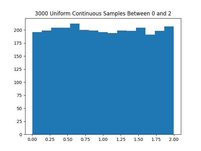
Here is a histogram using the above code generating 3000 samples between 0 and 2 using $m=3719$, $a=7$, and $R_0 = 1$.

Uniform discrete

To get discrete samples from a uniform distribution between $0$ and some positive constant $c$, we can simply mod our samples that we got from the MCG by $c$. We can do this because each of our samples are pseudo uniformly distributed between a higher number and modding will retain the pseudo uniformity. This can be implemented as follows:

uniform_samples = [i%c for i in samples]

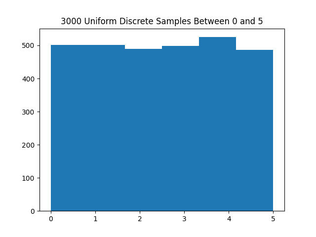
Here is a histogram using the above code generating 3000 samples between 0 and 5 inclusive using $m=3719$, $a=7$, and $R_0 = 1$.

Arbitrary discrete

To generate samples from an arbitrary discrete distribution, we can think of dividing up the interval between 0 and 1 by the probability of each of the x’s in our domain of the probability mass function $p(x)$. We can then return as a sample the interval that a uniform sample fell in to.

So for example, if we had a Bernoulli distribution defined by the probability of $x=0$ as $0.4$ and $x=1$ as $0.6$, then we would divide up the unit interval between 0 and 1 with $0$ to $0.4$ and $0.4$ to $1$. Then, we get a uniform sample $u$ between $0$ and $1$. If $u$ is in between $0$ to $0.4$, we return 0 as the sample. If $u$ is in between $0.4$ to $1$, we return 1 as the sample. To implement this, we can simply loop through each interval and see if a given sample curr_sample falls into the interval.

prev_boundary = 0
for j, bucket in enumerate(p):
    next_boundary = prev_boundary + bucket
    if curr_sample >= prev_boundary and curr_sample <= next_boundary:
        bucketed_samples.append(j)
        break

    prev_boundary = next_boundary

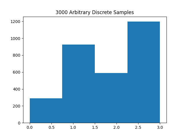
Here is a histogram using the above code generating 3000 samples for the pmf with $p(0) = 0.1$, $p(1) = 0.3$, $p(2) = 0.2$, and $p(3) = 0.4$ using $m=3719$, $a=7$, and $R_0 = 1$.

Conclusion

This post introduced pseudo random number generators with a specific example: Multiplicative Congruential Generators. Also presented were methods for sampling from discrete uniform and arbitrary distributions as well as continuous uniform distributions. All the code in the post is in this repository. Sampling from arbitrary continuous distributions is more complicated and will be covered in a later blog post. It involves methods called inverse cdf and rejection sampling.