
Unsupervised Feature Learning via Non-Parametric Instance Discrimination
A summary of the paper [Zhirong et al., 2018] as well as a mention of a followup paper MoCo [He et al., 2020] that builds upon the first.
Post Outline
- Intro
- General Methodology
- Softmax Formulation
- Results and Takeaways
- Supplementary Paper: Momentum Contrast for Unsupervised Visual Representation Learning
- Summary
- Resources
Intro
The problem that this paper is trying to solve is feature recognition in images in an unsupervised setting through feature representation. The paper approaches this problem via a non-parametric softmax formulation that maximizes distinction between instances. Essentially what the paper is trying to do is to come up with a framework that takes in a set of images and comes up with a consistent representation of each of them. These representations are close according to some metric if they look similar and far if they look different. We will go into the softmax formulation in more detail in a later section.
The motivation for this paper is the noticeable different in top 1 error and top 5 error in supervised approaches. The top 5 error is significantly smaller than the top 1 error, which the authors of the paper hypothesize that this is due to there being something that can be learned from the visual data themselves and not the semantic annotations.
General Methodology
Training
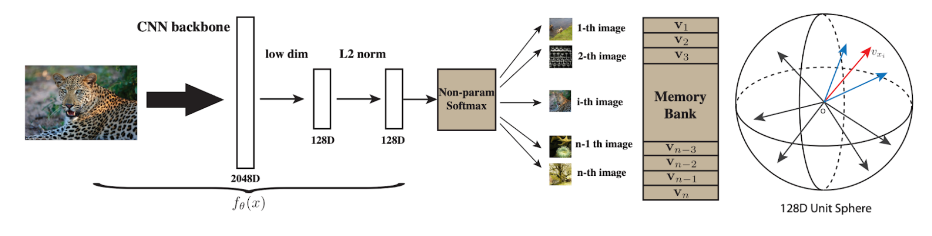
We want to learn a feature representation $f_\theta(x)$ that takes as input an image and outputs an 128 dimensional normalized vector. This vector is stored in a “Memory Bank” that contains all the vectors representing all the training images. We can view these vectors as being distributed in a 128 dimensional unit sphere. The parameters $\theta$ are updated through the objective functions that we will be covering next.
Classification
During classification, we compute the feature of a test image using $f_\theta(x)$ and perform classification using k nearest neighbors. The paper uses $k = 200$ and the cosine similarity as the distance function. This distance function makes sense if we view the vectors in the memory bank as being inside of a 128d unit sphere because cosine similarity computes the cosine of the angle between two vectors. The kNN vote is weighted according to the similarity between those closest 200 vectors and the input vector.
Softmax Formulation
The softmax function is the main part of the paper. We will go over the way the formulation was presented and add some commentary about why.
Take 1: Softmax Formulation
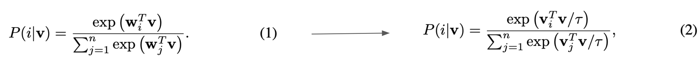
The main strategy the paper uses is instance discrimination. This basically means that the paper treats each image as its own class. In the case of Imagenet with 1000 classes and 1.2 million images, this means the paper will have 1.2 million classes. Because of this instance discrimination (which the paper uses) compared to class discrimination (traditional methods), we reformulate the softmax formulation. Equation 1 is the traditional softmax formulation that has a separate vector $w_i$ for each class while equation 2 has a separate vector $v_i$ for each image. In the case of Imagenet, this means there are 1000 $w$ vectors and 1.2 million $v$ vectors. From this, we can see why the model is non parametric. At a high level, non-parametric means that the number of parameters in the model scales with the amount of data.
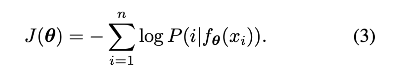
We formulate the objective function as the standard negative log likelihood function that we try to minimize.
Take 2: Noise Contrastive Estimation
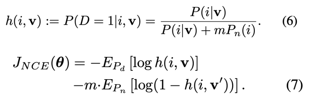
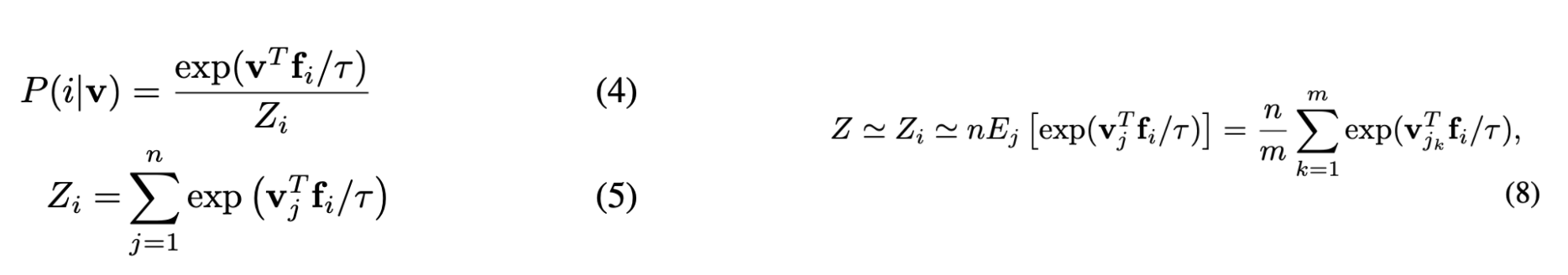
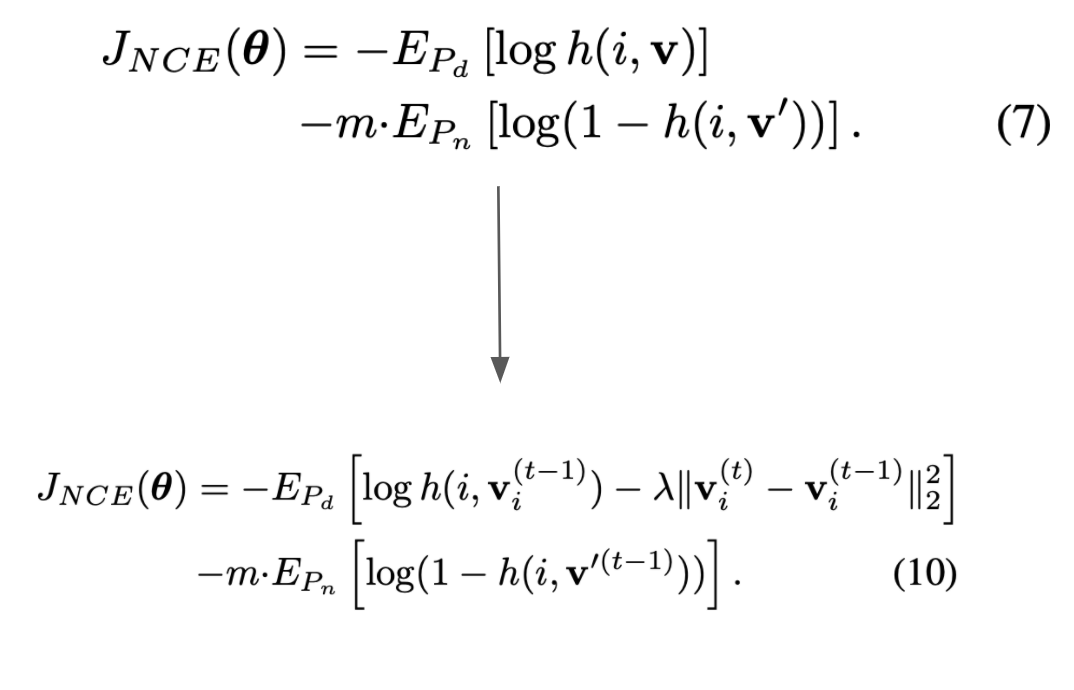
By treating each image as its own class and ending up with 1.2 million classes, we run into a computational problem. This is because defining the softmax as we did in equation 2 is infeasible to calculate at scale. Instead, the paper uses Noise Contrastive Estimation, a method of approximating the softmax in equation 2. The idea with Noise Contrastive Estimation is to reformulate the multi class classification task as a binary classification task. So instead of trying to distinguish between classes, we are trying to increase the probability that a sample $i$ with feature $v$ is from the data distribution $P_d$ and decrease the probability that the sample $i$ with feature $v’$ (feature vector for another image) is part of the data distribution. We end up with the following optimization objective in equation 7.
Where does the computational improvement actually come from? If we remember in equation 2, the denominator is the hard part because we have to sum over 1.2 million terms. Here, we use the Monte Carlo Integration formula in equation 8 to come up with an approximation for the numerator $Z_i$. We end up turning an O(n) calculation into an O(1) calculation per batch $j_k$ of the whole training set.
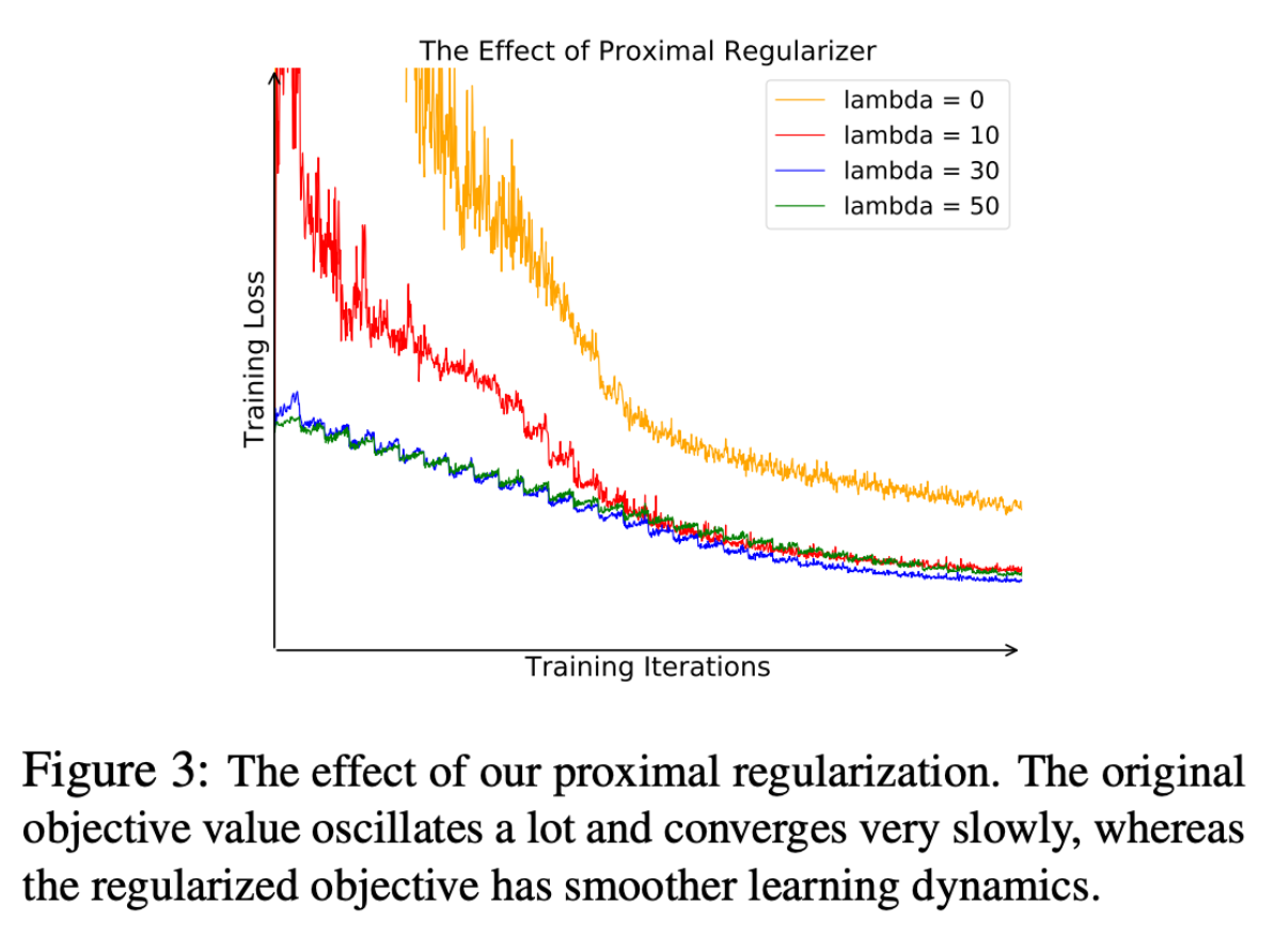
Take 3: Proximal Regularization
There is still another problem that comes up when we treat each image as a class. This formulation means that we only end up with one instance per class, which leads to a lot of fluctuation. The paper introduces a regularization term into the objective function (Equations 7 and 10), which leads to a decrease in oscillation as seen in Figure 3.
Results and Takeaways
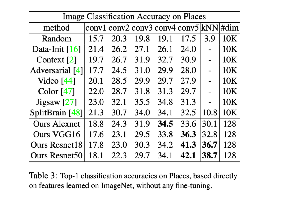
The results from the paper indicate that the presented framework outperforms other unsupervised methods by a large margin.
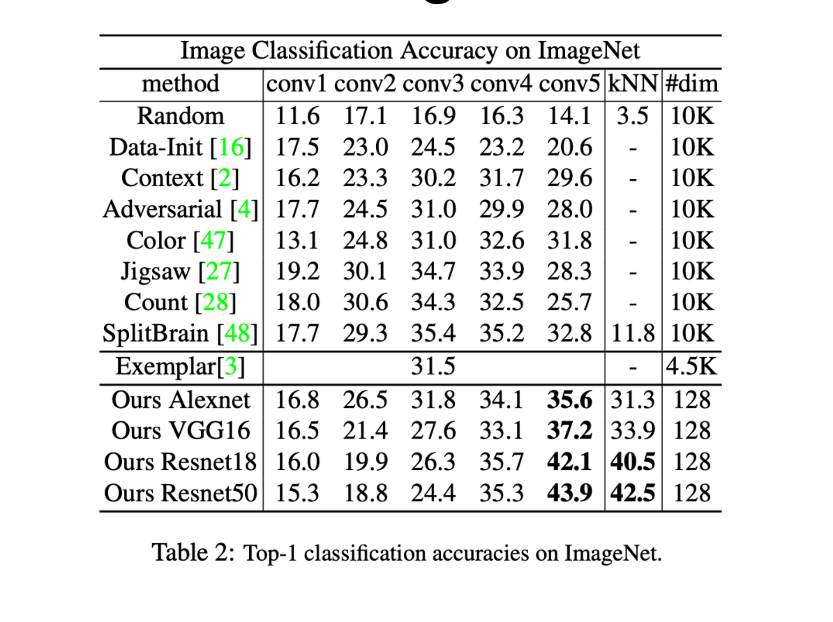
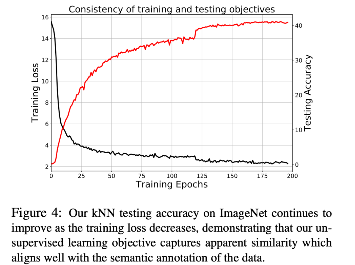
The table below also indicates that the capture similarity from the framework aligns well with the semantic annotation (i.e. class labels) of the data.
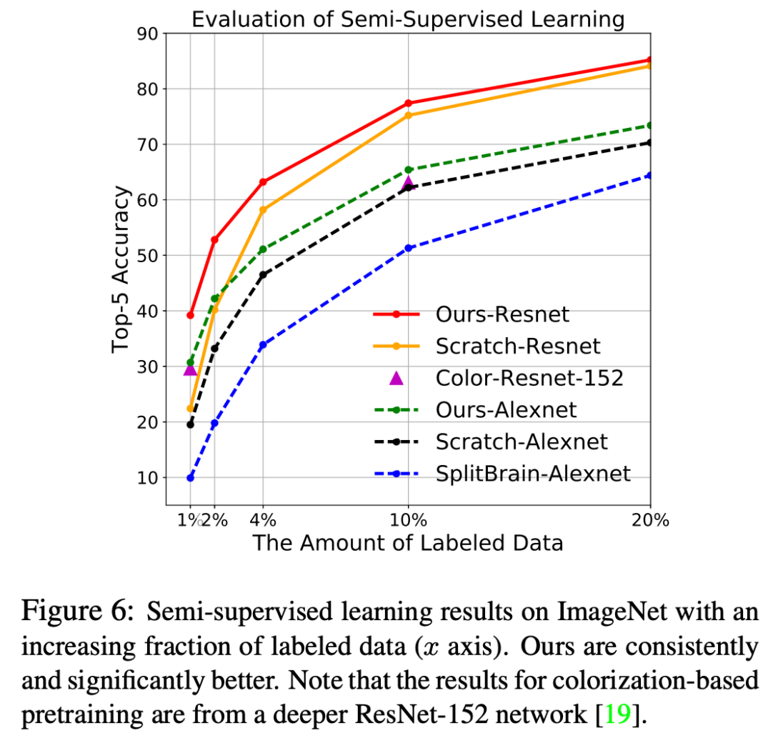
In the realm of semi supervised learning, the paper’s framework outperforms each of the presented methods (including supervised learning) up until 20% of the dataset is used as labeled data.
In transfer learning, the paper’s framework outperforms all the other unsupervised methods but still is worse than supervised learning by a significant margin.
Supplementary Paper:
Scaling is one of the key selling points of the previous paper. They were able to train on Imagenet, which consists of 1.2 million images, in only 600 megabytes. What if we wanted to scale to billions? The supplementary paper “Momentum Contrast for Unsupervised Visual Representation Learning” (aka MoCo) builds upon the main paper in this regard. We have the same task: unsupervised visual representation learning. We also have the same learning formulation: minimizing contrastive loss between instances.
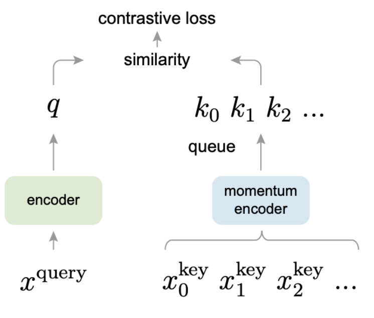
The idea is to build something called a “dynamic dictionary”. When we query an input from the dictionary, we expect to get a representation that is similar to our input. All the other stored feature vectors inside of the dictionary should be different. This part is similar to the main paper - images that look similar should be closer and images that look different should have a farther-apart representation inside the dictionary.
The dynamic part is what separates this model from the main paper’s model. “Dynamic” means that the dictionary is being trained on a continuously evolving subsample of the data. If we look at the figure below, we can see that there is a momentum encoder taking in subsets of the training data. The output of the momentum encoder is combined with the input encoder to calculate the contrastive loss that is then used for learning.
The paper presents a momentum function that decides the speed at which the subsample evolves. Evidently there is a sort of “dial” here where if we evolve too quickly, the model won’t be able to learn because it doesn’t have time to check (loses consistency). On the other hand, if we train to slowly, we’re only really training on that subset and nothing is really happening.
This presented method “MoCo”, outperforms the main paper’s method of utilizing a memory bank as seen below.
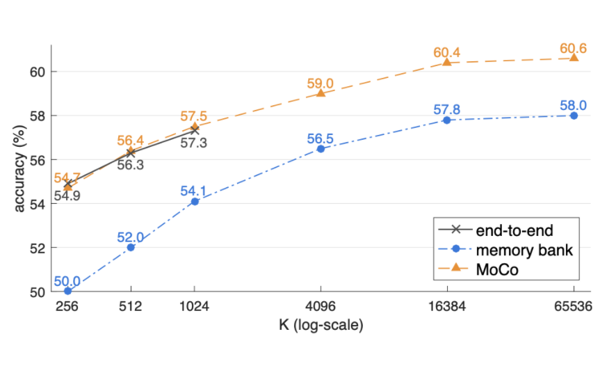
Because we are looking only at subsamples as opposed to the whole memory bank, we can scale even further. The paper experiments on Instagram’s billions scale dataset with noticeable improvement.
Summary
The main paper [Zhirong et al., 2018] presents an non-parametric instance discriminative framework for learning visual feature representations in an unsupervised setting. The followup paper [He et al., 2020] builds upon the main paper and scales to the billions.